


The displayed squared error is 0.000000 for the unconstrained fit but 4.000000 for the equality-constrained fit. I’m eager to dig into what a successful solver exit establishes: satisfied stopping criteria, not a model that fits your observations well.
Express the fitting target as the sum of squared prediction errors for your chosen slope and intercept. Discover how minimize uses your objective function and starting vector to return a candidate solution in an OptimizeResult.
What is SciPy minimize?
SciPy minimize searches for values that reduce a single numerical score using your objective function and starting vector, then returns an OptimizeResult containing the candidate solution and its termination details.
For a fitted line, the objective function converts your chosen slope and intercept into a scalar score by summing the squared prediction errors.
The input can contain several variables even though the output must be scalar. If array indexing is unfamiliar, the NumPy arrays tutorial explains how a coefficient vector stores those choices.
| Your problem | Starting interface | Boundary |
|---|---|---|
| Smooth objective without restrictions | minimize with BFGS | Uses gradient information, estimated when omitted |
| Individual variable limits | minimize with L-BFGS-B | Bounds restrict each variable separately |
| Relationships between variables | minimize with SLSQP | Supports equality and inequality constraints |
| One variable and no gradient interface needed | minimize_scalar | Takes a scalar variable rather than a coefficient vector |
| A vector of fitting residuals | least_squares | Accepts residuals directly instead of their summed square |
BFGS means Broyden-Fletcher-Goldfarb-Shanno and estimates curvature from gradient changes, while its limited-memory relative L-BFGS-B supports bounds. Sequential Least Squares Programming (SLSQP) handles relationships between variables.
SciPy selects BFGS, L-BFGS-B or SLSQP from the supplied restrictions when you omit method, without comparing algorithms on your objective.
Prerequisites for fitting a function
The examples use Python functions and NumPy arrays on Linux, with no administrator permissions required. The executed environment uses Python 3.14.8 with NumPy 2.5.3 and SciPy 1.18.1.
- A Python interpreter with virtual-environment support
- A terminal in a writable working directory
- NumPy and SciPy installed in the active environment
Create an isolated environment so the examples use their own packages rather than a system-wide installation, using the corresponding Scripts activation path on Windows.
python3 -m venv .tutorial-env
source .tutorial-env/bin/activate
python3 -m pip install numpy scipy
python3 -c "import sys, numpy, scipy; print(sys.version.split()[0]); print(numpy.__version__, scipy.__version__)"
The version command prints the interpreter followed by the two package versions, so it also confirms that imports reach the active environment. Save the following scripts beside one another because later examples import the objective and observations from the first file.
Fit and constrain a line with SciPy minimize
Use a small illustrative dataset with observations 1, 3, 5 and 7 at times 0, 1, 2 and 3. A line with slope 2 and intercept 1 fits these values exactly, giving you an independent answer to compare against the optimizer.
1. Define a scalar fitting loss
Save the following as fit_line.py, then run python3 fit_line.py. The coefficient vector starts at [0, 0], and args passes the fixed observations to each objective evaluation.
import numpy as np
from scipy.optimize import minimize

# Illustrative measurements, not an external dataset.
time = np.array([0., 1., 2., 3.])
observed = np.array([1., 3., 5., 7.])

def loss(coefficients, time, observed):
    slope, intercept = coefficients
    residual = slope * time + intercept - observed
    return float(residual @ residual)

result = minimize(
    loss, x0=[0., 0.], args=(time, observed), method="BFGS"
)

if __name__ == "__main__":
    print("success:", result.success)
    print("coefficients:", np.round(result.x, 6))
    print("squared error:", f"{result.fun:.6f}")
    print("message:", result.message)
    print("evaluations:", result.nfev)
SciPy supplies the changing coefficient vector as the first argument to loss, which is why that argument does not appear inside args. The residual array measures prediction minus observation, and its dot product with itself returns the single squared-error score.
I got [2, 1] from the unconstrained fit, and the displayed squared error rounded to zero. The numerical objective can still be a tiny positive value, so compare it with a tolerance rather than demanding exact floating-point equality.
Returning the residual vector changes the problem into one for least_squares, so keep the loss scalar. Replace time and observed with matching one-dimensional arrays for your data.
2. Supply the loss gradient
A gradient gives the change in loss for a small change in each coefficient. Here the slope derivative is twice the dot product of residual and time, while the intercept derivative is twice the residual sum.
Save this as compare_gradient.py and run python3 compare_gradient.py. The callback records the accepted iteration losses, and maxiter stops the optimization if it reaches the iteration budget.
import numpy as np
from scipy.optimize import minimize
from fit_line import loss, time, observed, result

def gradient(coefficients, time, observed):
    slope, intercept = coefficients
    residual = slope * time + intercept - observed
    return 2 * np.array([residual @ time, residual.sum()])

history = []
def record_progress(intermediate_result):
    history.append(float(intermediate_result.fun))

with_gradient = minimize(
    loss, [0., 0.], args=(time, observed), method="BFGS",
    jac=gradient, callback=record_progress,
    options={"gtol": 1e-8, "maxiter": 200}
)

if __name__ == "__main__":
    print("coefficients:", np.round(with_gradient.x, 6))
    print("numerical gradient evaluations:", result.nfev)
    print("analytic gradient evaluations:", with_gradient.nfev)
    print("callback losses:", np.round(history, 6))
    print("success:", with_gradient.success)
SciPy forwards args to the derivative as well as the objective, keeping their time and observed arguments aligned. Return the two gradient entries in coefficient order.
The numerical-gradient fit made 18 objective evaluations, while the analytic-gradient fit made 7 for these observations. Those counts describe this example, not a wall-clock benchmark or a guaranteed improvement on another function.
The callback parameter must be named intermediate_result for SciPy to pass an OptimizeResult with x and fun. Its recorded losses decreased from about 25.243375 to values that round to zero, but callback support and stopping behavior depend on the solver.
3. Add bounds and a coefficient relationship
A bound limits one coefficient independently, such as restricting the slope to the interval from 0 to 1.5. For a separate relationship example, require nonnegative coefficients with a sum of 2.
Save constrain_line.py beside the earlier scripts and run python3 constrain_line.py. Both calls use the same loss, letting the restrictions change the answer rather than silently changing the observations.
import numpy as np
from scipy.optimize import minimize
from fit_line import loss, time, observed
from compare_gradient import gradient

bounded = minimize(
    loss, [1., 1.], args=(time, observed), method="L-BFGS-B",
    jac=gradient, bounds=[(0., 1.5), (0., None)]
)
relationship = {
    "type": "eq",
    "fun": lambda coefficients: coefficients.sum() - 2.,
    "jac": lambda coefficients: np.ones(2)
}
constrained = minimize(
    loss, [1., 1.], args=(time, observed), method="SLSQP",
    jac=gradient, bounds=[(0., None), (0., None)],
    constraints=[relationship], options={"ftol": 1e-10, "maxiter": 200}
)

if __name__ == "__main__":
    for name, solution in [("bounded", bounded), ("constrained", constrained)]:
        print(name, "success:", solution.success)
        print(name, "coefficients:", np.round(solution.x, 6))
        print(name, "squared error:", f"{solution.fun:.6f}")
The bounds list follows coefficient order, and None leaves the intercept without an upper limit. SLSQP interprets the equality function as a residual that must be zero, so coefficients.sum() minus 2 expresses the required relationship.
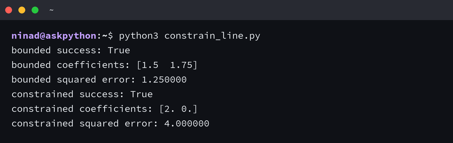
The unconstrained [2, 1] violates both the slope cap and the coefficient-sum requirement, which explains the increased fitting error. I used the same observations with both restrictions and got squared errors of 1.25 and 4.
For a dictionary inequality, SciPy requires the returned value to be nonnegative. Express a sum no greater than 2 as 2 minus the coefficient sum, not the reverse.
In portfolio optimization, a sum-of-weights relationship has a different interpretation from this illustrative fitting constraint. Choose the restriction from your model.
Verify the result and constraint residual
A successful solver exit reports that its stopping criteria were satisfied, which does not establish that the model fits your observations well. Read the termination message and evaluate the returned coefficients against the requirements you imposed.
Save the following as verify_fit.py and run python3 verify_fit.py. It recomputes both losses and checks the equality directly, with assertions that stop execution if the known answers are not met.
import numpy as np
from fit_line import loss, time, observed, result
from constrain_line import constrained

for name, solution in [("unconstrained", result), ("constrained", constrained)]:
    print(name, "success:", solution.success)
    print("message:", solution.message)
    print("finite:", bool(np.isfinite(solution.x).all() and np.isfinite(solution.fun)))
    print("recomputed loss:", f"{loss(solution.x, time, observed):.6f}")
    print("iterations:", solution.nit, "evaluations:", solution.nfev)

print("equality residual:", f"{constrained.x.sum() - 2.:.10f}")
print("predictions:", np.round(constrained.x[0] * time + constrained.x[1], 6))
assert result.success and np.allclose(result.x, [2., 1.], atol=1e-5)
assert constrained.success and np.allclose(constrained.x, [2., 0.], atol=1e-5)
assert abs(constrained.x.sum() - 2.) < 1e-7
| Measured result | Unconstrained fit | Equality-constrained fit |
|---|---|---|
| Coefficients | [2, 1] | [2, 0] |
| Displayed squared error | 0.000000 | 4.000000 |
| Solver iterations | 4 | 2 |
| Objective evaluations | 18 | 2 |
| Success | True | True |
The equality residual prints 0.0000000000, and the constrained predictions are [0, 2, 4, 6]. Each prediction is one below its observation, so four squared errors of 1 explain the loss of 4 without relying on the success flag.
An iteration can require several objective evaluations, so nit and nfev count different kinds of work.
For unfamiliar data, inspect residuals as well as the summed loss because different error distributions can produce the same score. The linear regression tutorial provides the statistical context that a numerical optimizer alone cannot supply.
Troubleshoot failed or misleading optimization
An optimizer can return a coefficient vector even when it has not converged. I stopped the solver after one iteration, and it returned a finite candidate with success set to False.
Save this as failed_fit.py and run python3 failed_fit.py to reproduce that state. The assertion accepts the intentionally failed optimization, so the script itself completes without disguising the solver failure.
import numpy as np
from scipy.optimize import minimize
from fit_line import loss, time, observed
from compare_gradient import gradient

limited = minimize(
    loss, [0., 0.], args=(time, observed), method="BFGS",
    jac=gradient, options={"maxiter": 1}
)
print("success:", limited.success)
print("message:", limited.message)
print("coefficients:", np.round(limited.x, 6))
print("squared error:", f"{limited.fun:.6f}")
print("iterations:", limited.nit)
assert not limited.success
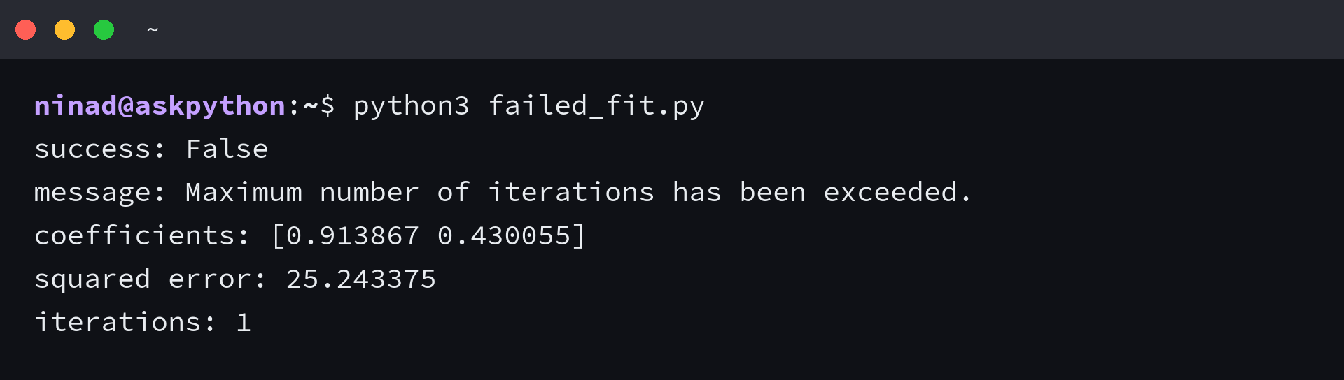
Increasing maxiter may let this smooth example finish, but that change cannot repair an incorrect objective or an impossible constraint. The failed candidate has a squared error of about 25.243375.
| Symptom | What to inspect | Action |
|---|---|---|
| Returns the initial guess | Does the loss change under small coefficient changes? | Remove accidental rounding or integer casts and inspect the gradient |
| Objective must return a scalar | Is the returned value a residual array? | Return its summed square or choose least_squares |
| Constraint remains violated | Sign, residual and feasibility of the constraint | Use zero for eq and nonnegative for ineq, then test a feasible point |
| Precision-loss message | Finite-difference accuracy and coefficient scales | Check analytic derivatives and method-specific tolerances |
If your program returns the initial guess, a piecewise-constant objective can hide changes from a finite-difference derivative. Choosing Nelder-Mead avoids derivative estimation, but it does not make a discontinuous or noisy objective reliably solvable.
The tol argument sets relevant solver-specific stopping tolerances, while options lets you control individual criteria. BFGS uses gtol for its gradient criterion, and SLSQP uses ftol in its optimality and feasibility tests, so one tolerance number does not define the same guarantee across methods.
L-BFGS-B uses a projected-gradient test that accounts for active bounds, which means an accepted boundary solution can have a nonzero ordinary gradient. Its workers option can parallelize numerical differentiation, but it does not parallelize the whole optimization or help this analytic-gradient example.
Consult the L-BFGS-B options or SLSQP options before applying a setting from another method. Accepted signatures are in the minimize reference.
Change the starting point before trusting a minimum
The fitted-line loss is a convex quadratic with a unique minimum because the observation times identify both coefficients. A different custom objective can have several local minima, so one successful run need not identify the lowest value across its domain.
Compare starting vectors without changing the objective by saving multiple_starts.py and running python3 multiple_starts.py. For a nonconvex extension, retain successful candidates and compare their scores and feasibility.
import numpy as np
from scipy.optimize import minimize
from fit_line import loss, time, observed
from compare_gradient import gradient

for start in ([0., 0.], [10., -10.], [-5., 8.]):
    candidate = minimize(
        loss, start, args=(time, observed), jac=gradient, method="BFGS"
    )
    print("start:", start, "success:", candidate.success,
          "coefficients:", np.round(candidate.x, 6))
    assert candidate.success and np.allclose(candidate.x, [2., 1.], atol=1e-5)
All three starts converged to coefficients within the asserted tolerance of [2, 1]. For a nonconvex objective, agreement across selected starts is useful evidence rather than proof of a global minimum, and a global solver such as differential_evolution serves a different search task.
Frequently asked questions
A one-variable objective still needs a scalar return value, but a scalar return value can come from an objective with several variables. Choose the interface from the inputs and restrictions.
What is tol in SciPy minimize?
The tol argument sets a termination tolerance that the selected solver maps to relevant stopping criteria. Use method-specific options when you need control over an individual criterion, and evaluate accuracy against your application separately.
Can scipy.optimize.minimize handle integer variables?
It optimizes continuous variables and does not enforce integer decisions. Rounding the returned vector can violate constraints or change the objective, so formulate a mixed-integer problem with an appropriate solver such as scipy.optimize.milp when the model is linear.
Does SciPy minimize find every local minimum?
A single call searches from one starting point and returns one candidate. It does not enumerate local extrema or certify a global minimum for an arbitrary nonconvex function.
When should I use minimize_scalar instead of minimize?
Use minimize_scalar for a one-variable scalar objective when its available methods match the problem. Use minimize with a one-element vector when you need its gradient interface or general constraint machinery.
Does least_squares minimize root mean squared error?
With its default linear loss, least_squares minimizes half the sum of squared residuals. For a fixed number of residuals, that has the same minimizers as root mean squared error, but the reported cost is not that error metric.
