

Using historical data to confirm performance improvements turns a fast test into evidence the business can defend.
Using historical data to confirm performance improvements starts with one fair question. Did the same work become cheaper under comparable conditions? In an illustrative case, a DBA deploys an index at 9:00 AM and watches average reads fall. The release channel fills with check marks.
Before deployment, the query averaged 42,000 logical reads across 18,400 executions. Afterward, it averaged 6,100 reads across 11,200 executions. Total reads fell 91 percent, but executions fell 39 percent too.
That missing context changes the decision. The team now needs matched windows, stable plans, and comparable parameters. Enough executions must pass before anyone calls the index a success.
One Fast Execution Proves Almost Nothing
A clean test confirms a change for one parameter set. It cannot represent every customer, data distribution, or concurrency pattern. Cached pages and quiet servers can flatter results while hiding blocking, memory pressure, or storage latency.
Start with per-execution duration, CPU, logical reads, writes, and waits. Then add execution count. If executions double after latency halves, aggregate duration stays level. Total CPU and reads still require separate calculations.
Both views matter because users experience individual calls, while servers absorb the complete workload. Application growth may raise daily CPU despite better per-call latency. Modest per-call gains may also save substantial capacity on frequent statements. Report both perspectives instead of selecting the flattering number.
Use a Before-and-After Scorecard
| Measure | What to Compare |
|---|---|
| Duration | Typical behavior and slow outliers |
| CPU and reads | Per execution and total workload |
| Executions | Count, application, and parameter mix |
| Plan | Plan identity and estimate quality |
| Writes | DML latency, log volume, and maintenance |
Build Comparable Workload Windows
Compare Monday morning with another normal Monday morning, not Sunday night. Match business cycles, batch schedules, release activity, and expected traffic. Keep important database, hardware, and configuration conditions consistent.
The plan may change when a large customer replaces a small one. Match applications, databases, users, query signatures, and parameter patterns. Note any statistics update or plan change inside either window.
Use several windows when the workload varies naturally. One favorable hour may be noise, while repeated improvements establish a pattern. Include enough executions to limit isolated outliers, and preserve the exact deployment time.
Normalize totals when windows cover different durations, but never hide the raw values. Rates per minute help compare uneven windows, while counts preserve capacity impact. Separate scheduled jobs from interactive traffic when their patterns differ. Otherwise, one overnight process can make a healthy daytime change look unsuccessful.
Read Product History With Context
SQL DM from IDERA charts query history for average duration, CPU, reads, writes, waits, blocking, deadlocks, and CPU per second. Event occurrences add execution-level statistics and SQL text. Now the graph answers the useful question: did the query stay faster during real traffic?
That history still reflects collection settings. Filters, thresholds, disabled monitoring, and retention choices can create gaps. Older query records may be aggregated into daily summaries, which suppresses some statement, client, and user detail. Repository grooming can also remove data beyond the configured retention period.
Use Query Store as a Second Witness
Query Store persists query text, plans, and runtime statistics. SQL Server 2017 and later can capture query-level waits. This historical evidence can connect an improvement with an index, plan, or workload change.
Query Store is not a recording of every execution. Runtime statistics are aggregated into configurable time intervals. Its averages, minimums, maximums, and standard deviations describe each plan within those intervals. Capture policies, cleanup settings, and storage limits determine what remains available.
Compare plan identifiers as well as query identifiers, because lower duration may come from an unrelated new plan. A forced plan or statistics refresh may alter the result. The claim gets stronger when the plan, change, and result share one clear timeline.
Measure the Cost of the Improvement
An index can reduce reads for selected queries while increasing work for data changes. Check insert, update, and delete activity on the affected table. Review index size, maintenance time, logging, lock behavior, and storage consumption. Confirm that neighboring queries did not regress.
Native index usage counters can reveal seeks, scans, lookups, and update maintenance. However, those counters reset after events such as a server restart. Record the observation start time, because a short window may miss monthly reports depending on the index.
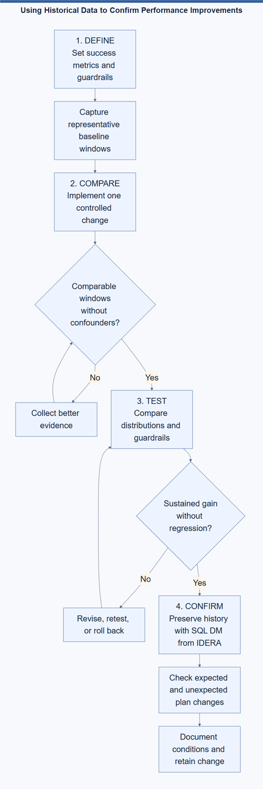
Define success and guardrails before deployment, such as lower reads without raising write latency beyond an agreed threshold. Capture the same metrics after deployment for an equivalent business window. Keep a rollback script available until the evidence remains stable.
The Fair Counterargument
Controlled benchmarks can demonstrate causality better than messy production history. A test regression costs nothing, while a production regression costs customers. That argument holds when test data and execution conditions represent production. Laboratory testing makes repeated measurements safer, especially when schema changes carry real risk.
However, controlled tests remove the concurrency, parameter diversity, and operational surprises that often determine production performance. Historical monitoring supplies that missing context. The strongest conclusion combines controlled testing with comparable production windows. Neither source should carry the decision alone.
A Result Worth Keeping
Baselines provide a comparison. SQL DM from IDERA supports a moving seven-day dynamic baseline and fixed custom periods. Choose normal periods and exclude quiet hours that distort expected behavior. A baseline is a reference, not an automatic verdict.
A trustworthy report shows the gain and every reason it might be misleading. Name the change, workload window, execution count, plans, and resource effect. Document competing deployments, missing data, and the period of stable behavior.
The DBA from 9:00 AM should wait through the next comparable peak. If reads stay lower and the guardrails hold, the change has earned its place. Then write the result down, because next quarter nobody will remember the details.
A fast test opens the case. A faster workload earns the decision.
Reference: Pinal Dave (https://blog.sqlauthority.com/), X
